Introduction:
Performing arithmetic operations in Excel is not only easy but also intuitive. When it comes to multiplication, Excel offers two main methods: using the multiplication operator (asterisk *) and employing the PRODUCT function. In this comprehensive guide, we will explore the step-by-step process of mastering Excel’s formula for multiplication.
You can download the Full Excel Sheet As Your Refference: Download Link Given Below
1.Using the Multiplication Operator (*):
This method is straightforward and commonly used for basic multiplication operations in Excel. It’s suitable for multiplying individual cells or values.
Let’s say you have the values 5 in cell A2 and 8 in cell B2. Follow the steps given below to multiply these values using the multiplication operator (*):
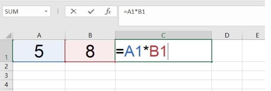
- Step 1: Select the cell where you want the result (e.g., C2).
- Step 2: Type the formula in C2: =A1*B1
- Step 3: Press Enter To get the Result.
The result will be displayed in the selected cell (C1), showing the product of 5 and 8, which is 40.
How to Use the Percentage Formula in Excel: Step-by-Step Process To Calculate Percentage of Total In Excel
Excel Formulas
2.Using the PRODUCT Function:
This method is useful when you want to multiply a range of values in Excel. The PRODUCT function calculates the product of all the numbers in a given range.
Let’s say you have the values 2, 3, 4, 5, and 6 in cells A1 to A5. Follow the steps below to multiply these values using the PRODUCT function:
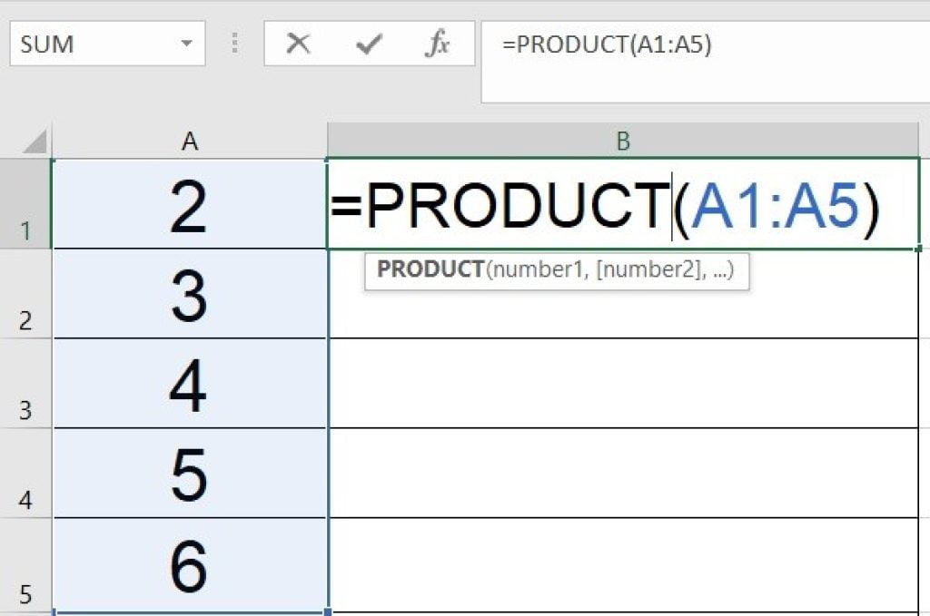
- Step 1: Select the cell where you want the result (e.g., B1).
- Step 2: Type the formula in B1: =PRODUCT(A1:A5)
- Step 3: Press Enter to get the result.
The result will be displayed in the selected cell (B1), showing the product of 2, 3, 4, 5, and 6, which is 720.
This method is particularly handy when dealing with multiple data points and wanting to find the product of an entire range.
3.Using the SUMPRODUCT Function:
The SUMPRODUCT function in Excel is a versatile tool that allows you to multiply corresponding elements in arrays and then sum up the results. This makes it a powerful choice for more complex multiplication scenarios.
Let’s say you have values 2, 3, 4, 5, and 6 in cells B1 to B5, and 1, 2, 3, 4, and 5 in cells C1 to C5. Follow the steps below to multiply and sum these corresponding values using the SUMPRODUCT function:
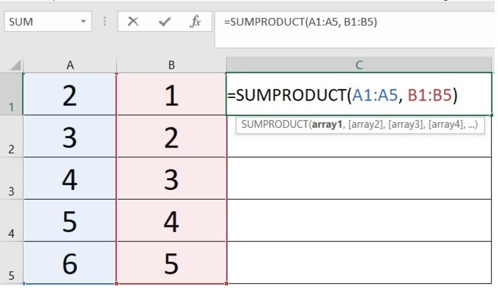
- Step 1: Select the cell where you want the result (e.g., D1).
- Step 2: Type the formula in D1: =SUMPRODUCT(B1:B5, C1:C5)
- Step 3: Press Enter to get the result.
The result will be displayed in the selected cell (D1), showing the sum of the products of corresponding elements, which is 70.
The SUMPRODUCT function is particularly useful for more advanced multiplication scenarios involving arrays of data.
Free Download
4.Array Formulas for Element-Wise Multiplication:
Array formulas in Excel allow you to perform element-wise operations on arrays of data. In the context of multiplication, this means you can multiply corresponding elements in two ranges.
Let’s say you have values 2, 3, 4, 5, and 6 in cells A1 to A5 and 1, 2, 3, 4, and 5 in cells B1 to B5. Follow the steps below to multiply these corresponding values using an array formula:
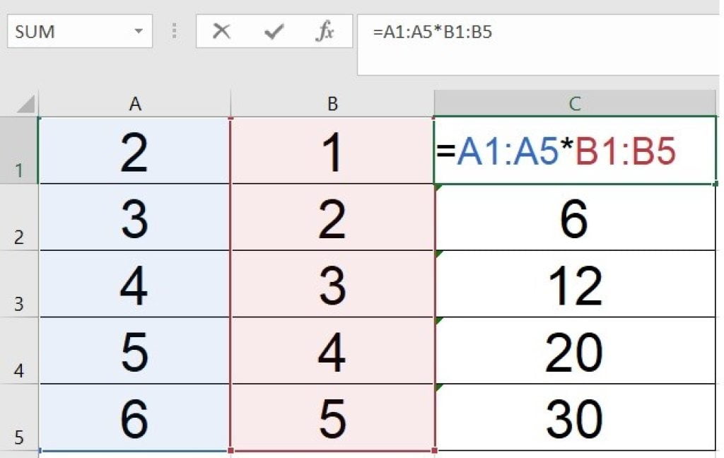
- Step 1: Select the cell where you want the result (e.g., C1).
- Step 2: Type the formula in C1: =A1:A5*B1:B5
- Step 3: Press Ctrl+Shift+Enter to finalize the array formula.
The result will be displayed in the selected cell (C1), showing the element-wise product of the corresponding values, which is 2, 6, 12, 20, and 30.
5.Using the Power Function (^):
The Power Function in Excel, represented by the caret (^) symbol, is useful when you need to perform calculations involving powers and exponents.
Let’s say you have the value 3 in cell A1. Follow the steps below to square this value using the Power Function:
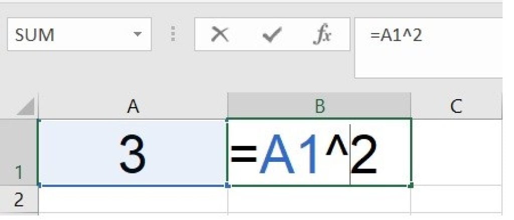
- Step 1: Select the cell where you want the result (e.g., B1).
- Step 2: Type the formula in B1: =A1^2
- Step 3: Press Enter to get the result.
The result will be displayed in the selected cell (B1), showing the square of the value in cell A1, which is 9.
Biography of Homi Jehangir Bhabha: The Visionary Scientist Who Changed the World
Read Biography
6.Paste Special for Constant Multiplication:
The Paste Special feature in Excel allows you to perform various operations, including multiplication by a constant, on a selected range.
Let’s say you have a constant value 10 in cell D1, and you want to multiply it by the values in cells A1 to A5. Follow the steps below:
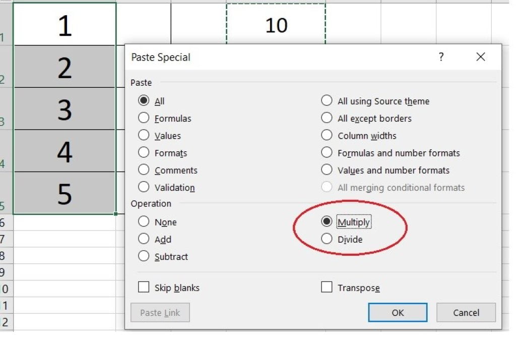
- Step 1: Enter the constant in an empty cell (e.g., D1).
- Step 2: Copy the constant by selecting D1 and pressing Ctrl+C.
- Step 3: Select the range you want to multiply (e.g., A1 to A5).
- Step 4: Right-click on the selected range, choose “Paste Special.”
- Step 5: In the Paste Special dialog, select “Multiply.”
- Step 6: Click OK.
The result will be the values in the selected range (A1 to A5) multiplied by the constant value (10).
Using Paste Special for Constant Multiplication is efficient when you need to scale an entire range by a constant factor.
The Hidden Power of Daily Habits: Shaping a Positive Well-Being
Self Development
7.Direct Cell References:
Direct cell references in Excel allow you to multiply a specific cell by a constant or another cell value.
Let’s say you have the value 7 in cell A1, and you want to multiply it by a constant, say 5. Follow the steps below:
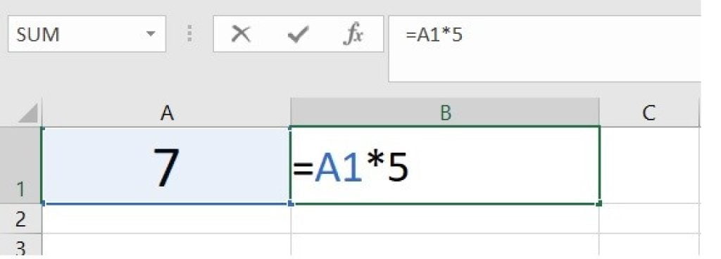
- Step 1: Select the cell where you want the result (e.g., B1).
- Step 2: Type the formula in B1: =A1*5
- Step 3: Press Enter to get the result.
The result will be displayed in the selected cell (B1), showing the product of the value in cell A1 (7) multiplied by the constant (5), which is 35.
Direct cell references are useful for basic multiplication tasks where you want to multiply a specific cell by a constant.
8.Utilizing COLUMN or ROW Functions:
The COLUMN and ROW functions in Excel can be employed for position-based multiplication, allowing you to perform calculations based on the position of a cell within a row or column.
Let’s say you have the value 6 in cell A1. Follow the steps below to multiply it by its column number:
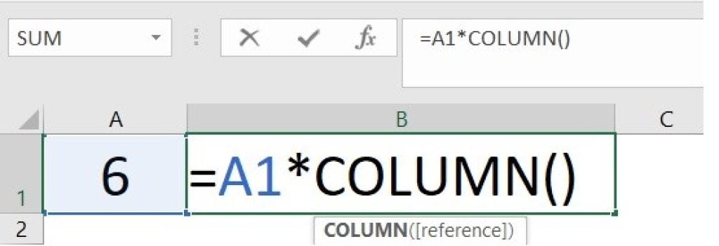
- Step 1: Select the cell where you want the result (e.g., B1).
- Step 2: Type the formula in B1: =A1*COLUMN()
- Step 3: Press Enter to get the result.
The result will be displayed in the selected cell (B1), showing the product of the value in cell A1 (6) multiplied by its column number.
Utilizing COLUMN or ROW functions is useful when you need calculations based on the position of the cell within a row or column.
Atomic Habits Summary Decoded: Positive Changes for a Powerful Life
Free Book Summary
Conclusion
Excel offers versatile methods for multiplication, catering to various scenarios. Whether using the asterisk, cell references, or specialized functions like PRODUCT, Excel empowers users to perform accurate and efficient multiplication operations. Feel free to download the practice file provided to grow your skills and become more proficient in multiplying in Excel.


