Introduction to conditional formatting in excel
Are you getting stuck in the sea of numbers and data in your Excel spreadsheets? Don’t worry! conditional formatting in Excel is here to transform your data tables into visually appealing and insightful masterpieces. In this guide, we’ll walk you through the steps using a practical example – a sales performance data table. Let’s dive in and discover how to make your data speak volumes!
Why Use Conditional Formatting in Excel?
Conditional formatting is like the artist’s palette of Excel. It allows you to highlight specific data points based on conditions you set, making trends and insights leap off the screen. In the example, we’ll use a sales performance data table to showcase the power of Conditional Formatting features.
Learn Excel Formulas
Step 1: Prepare your data table and Logics.
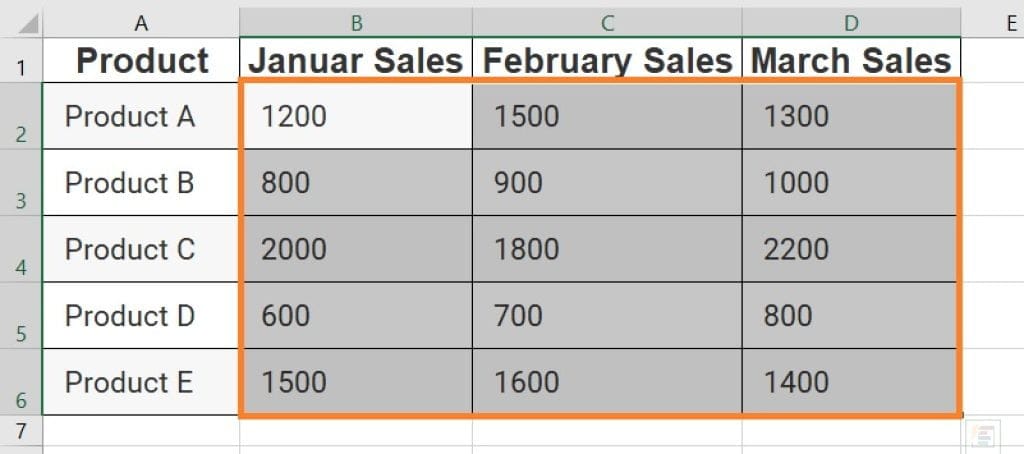
For example purpose we are using the below mentioned data table, where it is displaying Monthly sales figures for each product. In this table we want to highlight sales figures Greater Than 1500, Between 1000 and 1500, Less Than 1000.
| Product | January Sales | February Sales | March Sales |
| Product A | 1200 | 1500 | 1300 |
| Product B | 800 | 900 | 1000 |
| Product C | 2000 | 1800 | 2200 |
| Product D | 600 | 700 | 800 |
| Product E | 1500 | 1600 | 1400 |
Excel Formulas
Step 2: Select Your Data Table
Select the full sales data table, including the product names and monthly sales figures, To apply conditional formatting in excel, as shown in the picture.
Step 3: Go to “Home” Tab
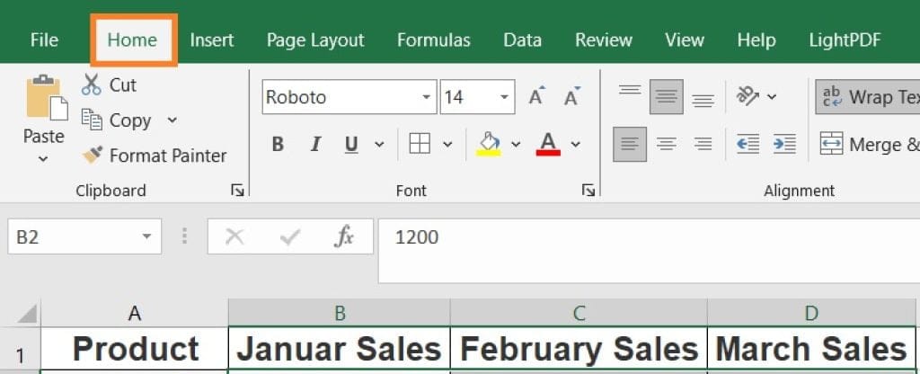
Navigate to the “Home” tab on the Excel ribbon, as shown in the below photo.
Free Resources
Step 4: Click “Conditional Formatting”
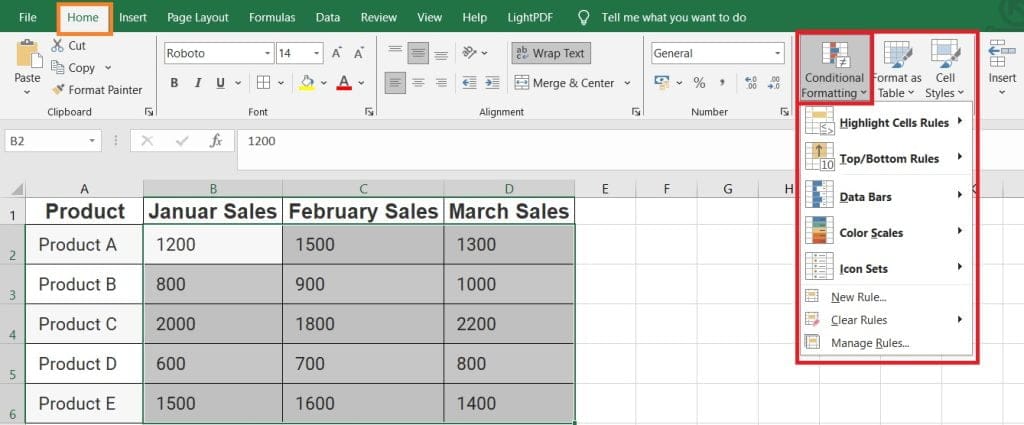
Locate and click on the “Conditional Formatting” option in the ribbon. A drop-down menu will appear.
Step 5: Choose “Highlight Cells Rules”
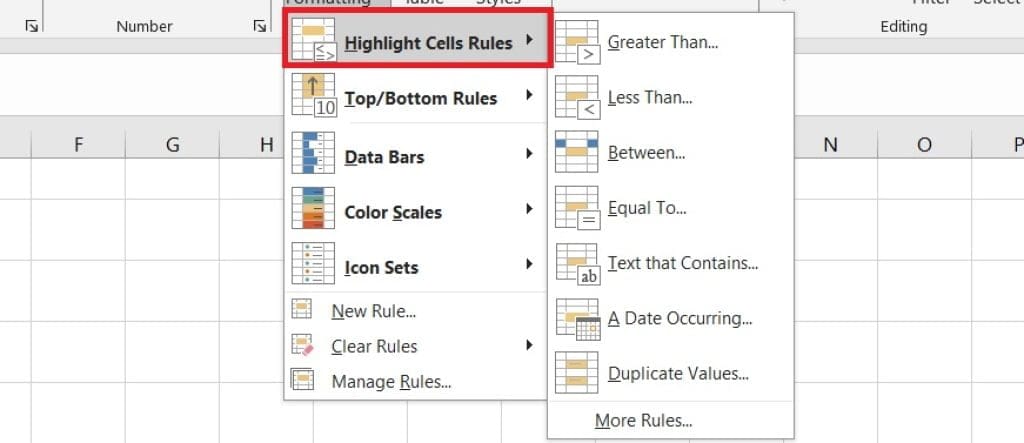
From the drop-down menu, choose “Highlight Cells Rules.” Here, you’ll see various options for setting conditions.
Cheat Sheets
Step 6: Set Conditions for High Sales
- Select “Greater Than” Rule Option From The Highlight Cells Rules.
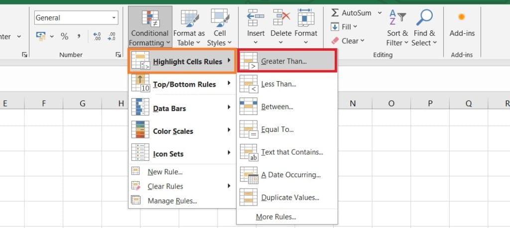
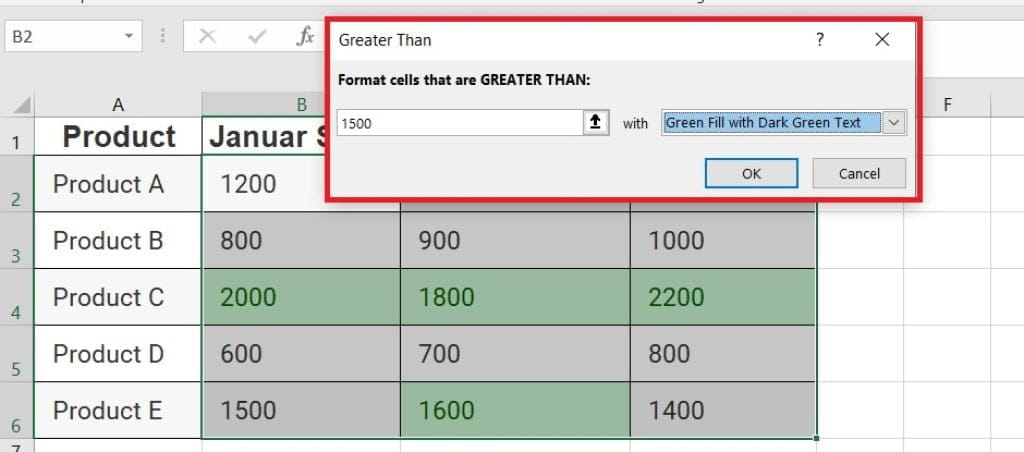
- Enter 1500 In the dialog box. This will highlight cells where sales are above 1500 units with a green fill. Then click on “OK.”
Step 7: Set Conditions for Moderate Sales
- Choose “Between” Rule Option From The Highlight Cells Rules.
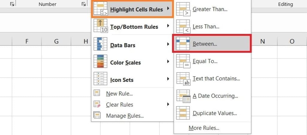
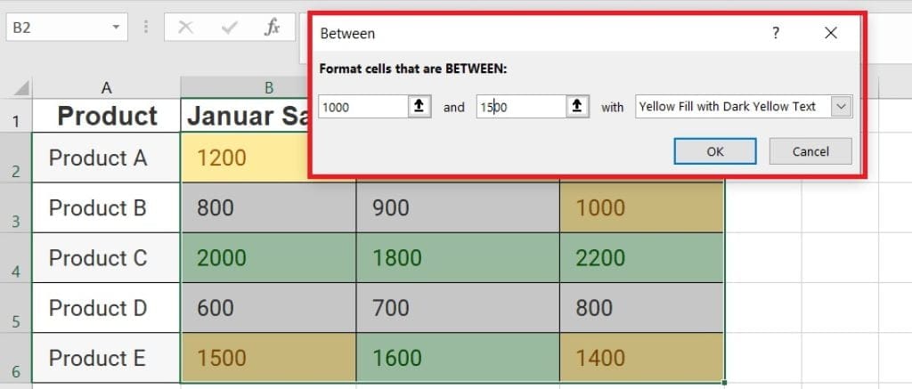
- Then Enter 1000 as the minimum and 1500 as the maximum. Apply a yellow fill to represent moderate sales. Click “OK.” to apply the condition.
Step 8: Set Conditions for Low Sales
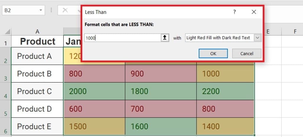
- Choose “Less Than” Rule Option From The Highlight Cells Rules.
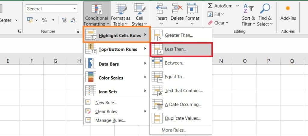
- Then enter 1000 in the Less than field. This will highlight cells with sales below 1000 units in red. Click “OK.” to apply.
Shortcut PDF Download
Step 9: Preview and Apply Formatting
Excel will show a preview of how the formatting will appear. Confirm the settings and click “OK” to apply the conditional formatting to your selected data range.
Step 10: Analyze the Results
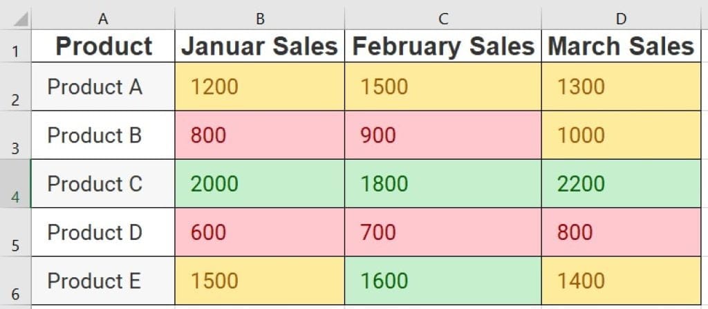
Behold the transformed sales data table! Green cells represent high sales, yellow cells indicate moderate sales, and red cells highlight low sales. With just a glance, you can identify the products and months that stand out.
Best 19 Attendance Sheet For Excel : Free Download Attendance sheet in excel
Free Templates
Conclusion
Conditional formatting in Excel is your secret weapon for making sense of complex data. By applying these simple steps to our sales performance example, you’ve now mastered the art of making your data visually appealing and insightful. Experiment with different rules and conditions to customize your Excel tables and unveil meaningful patterns,Thank You.
Exam Preparation


