Introduction:
When it comes to financial calculations, understanding the concept of simple interest is essential. In this article, we will explore how you can use Google Sheets to calculate simple interest effortlessly.
Whether you’re a student learning about interest or a professional managing finances, mastering the simple interest formula will prove invaluable. So let’s dive in and discover how to leverage Google Sheets to calculate simple interest with ease.
Understanding Simple Interest Formula
Simple interest is a fundamental concept in finance that helps us calculate the amount of interest earned or paid on a loan or investment. Unlike compound interest, which takes into account the accumulated interest over time, simple interest only considers the initial principal amount.
Formula: The formula for calculating simple interest is straightforward: I = P * R * T
Where:
- I represents the interest amount
- P is the principal amount (the initial sum of money)
- R denotes the rate of interest
- T represents the time period (in years)
Example:
Let’s say you have a principal amount of ₹1,000, with an annual interest rate of 5%, and you want to calculate the simple interest after 3 years.
Using the formula:
I = P * R * T
= ₹1,000 * 0.05 * 3
= ₹150
In this example, after three years, you would earn ₹150 in simple interest on your initial investment of ₹1,000.
Understanding how to apply the simple interest formula allows you to make informed financial decisions. Whether you’re borrowing money or investing it, knowing how much interest you’ll be paying or earning helps you plan and manage your finances effectively.
Setting Up Your Google Sheet
Now that you understand the concept of simple interest, let’s dive into setting up your Google Sheet to calculate it efficiently. Follow these steps to get started:
Creating a New Sheet:
- Open Google Sheets URL in your web browser.
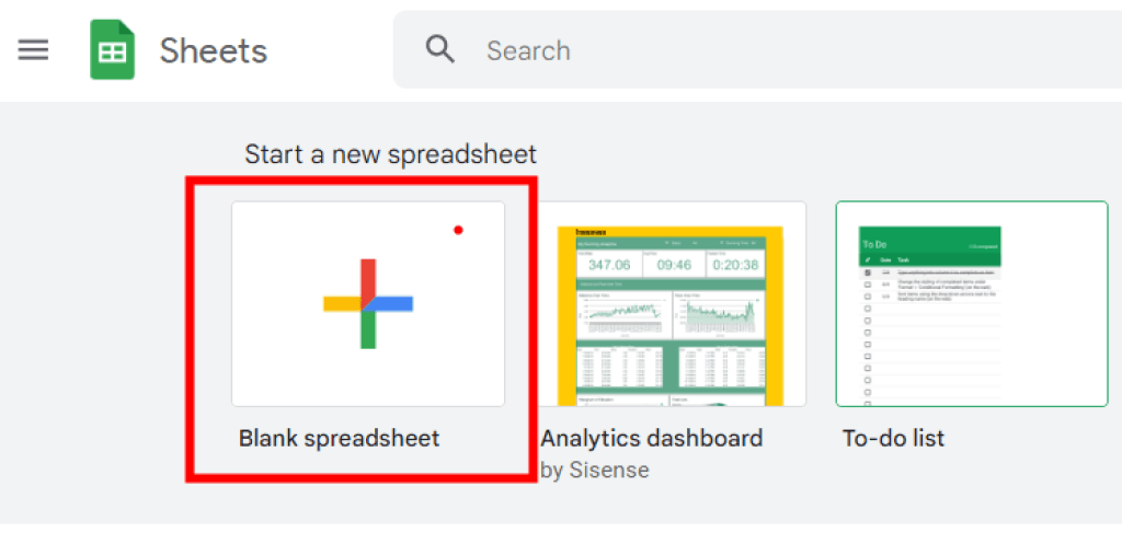
- Click on the “+ Blank” button to create a new spreadsheet, A new blank sheet will open
- Rename The Sheet by Click on the default sheet name if required.
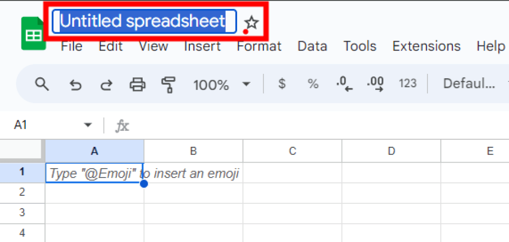
- Now you are ready to input your data in the sheet.
Free Templates
Entering Data:
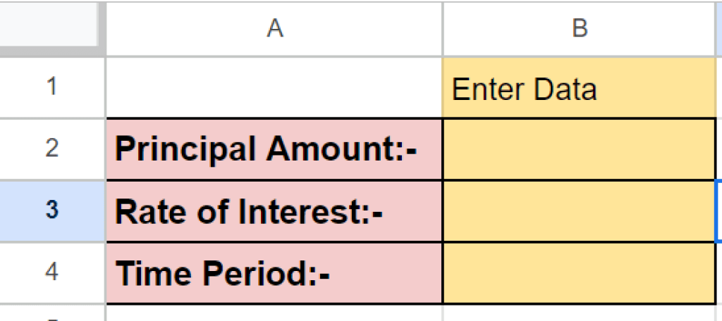
- In the first column, label the cells for Principal Amount, Rate of Interest, and Time Period.
- In the second column, enter the respective values for each category.
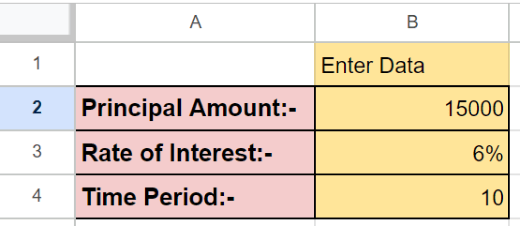
For example, in cell A2, enter “Principal Amount,” and in cell B2, enter the actual principal amount you want to calculate the interest for.
How to Effectively Recover Google Account: Step-by-Step Guide
Account Recovery
Formatting Cells:
- To improve readability and accuracy, you can format cells accordingly.
- Select the range of cells containing the values (e.g., B2).
- Right-click and choose “Format cells” from the context menu.
- In the Format sidebar, select your desired formatting options such as currency or decimal places.
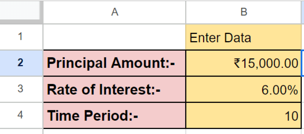
By setting up your Google Sheet with labeled cells and formatted data, you create a clear structure for calculating simple interest. In the next section, we’ll explore how to use formulas in Google Sheets to calculate simple interest effortlessly.
Professional Gmail Signature: Learn How to Make a Signature in Gmail
Gmail Setup
Calculating Simple Interest using Formulas
Now that your Google Sheet is set up with the necessary data, it’s time to calculate the simple interest using formulas. Follow these steps:
Using Multiplication Operators:
- Select an empty cell where you want to display the calculated interest amount, (i am entering in B5).
- In that cell, enter the formula “=P * R * T“, replacing P, R, and T with the respective cell references.
- For example, if the principal amount is in cell B2, the rate of interest is in cell B3, and the time period is in cell B4, the formula would be “=B2 * B3 * B4“.
- Press Enter to calculate the simple interest.
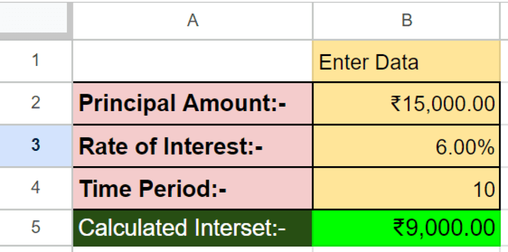
Benifits of Cell References:
- Instead of using hard-coded values in your formula, it’s best to use cell references.
- Cell references allow for flexibility and ease of updating values without modifying the formula itself.
For example, if you decide to change the principal amount from ₹1,000 to ₹2,000, you can simply update cell B2 with ₹2,000, and the formula will automatically recalculate.
Productivity Tools
Auto-fill Feature:
- If you have multiple rows of data for which you want to calculate simple interest, you can use the auto-fill feature in Google Sheets.
- After entering the formula in one cell (e.g., C2), hover over the bottom-right corner of that cell until a blue square appears.
- Click and drag down to auto-fill the formula for all rows that contain data.
- Google Sheets will adjust the cell references accordingly for each row.
Rounding Off:
Depending on your preference or specific requirements, you may want to round off the calculated simple interest amount.
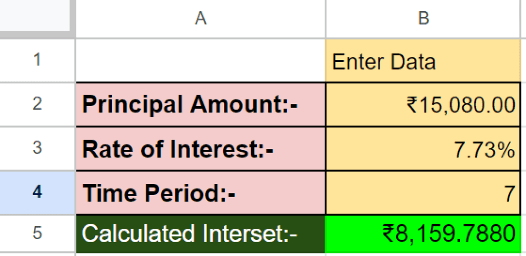
To do this, select the cells containing the calculated interest amounts and apply your desired rounding off option from the toolbar.
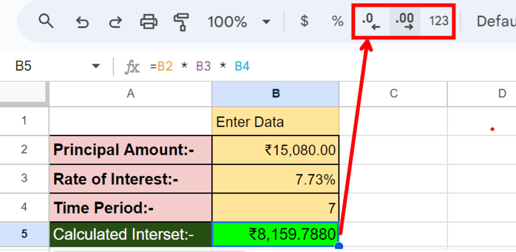
By following these steps, you can easily calculate simple interest using formulas in Google Sheets.
All Shortcuts PDF
Online Tools To Calculate Simple Interest
There are so many online tools available to calculate Simple Interest, that simplify the process and provide accurate results. Some of them are mentioned below, you can use those tools for free.
- Simple Interest Calculator By Grow.
- Simple Interest Calculator By Bajaj Finance.
- Simple Interest Calculator By Tax2Win.
- Simple Interest Calculator By IND Money.
- Simple Interest Calculator By ET Money.
Conclusion:
Congratulations! You have now learned how to understand and calculate simple interest using Google Sheets. By setting up your sheet, entering data, and applying formulas, you can effortlessly calculate simple interest for various scenarios.
Remember to practice and explore further with Google Sheets’ features to become more proficient in calculating simple interest. With this knowledge, you’ll be better equipped to manage your finances effectively and make informed decisions regarding loans, investments, or savings.
FAQ’s
Q1. What is the formula for interest in Google Sheets?
A1: The formula for interest in Google Sheets is “=P*R*T“, where P is the principal amount, R is the annual interest rate, and T is the time period in years.
Q2. How do I calculate simple interest?
A2: To calculate simple interest, use the formula “I = P * R * T“, where I is the interest, P is the principal amount, R is the interest rate, and T is the time period in years.
Q3. What is the formula for interest in Excel?
A3: The formula for interest in Excel is “”=P*R*T“, similar to Google Sheets. P represents the principal amount, R represents the annual interest rate, and T represents the time period in years.
Q4. How do you calculate interest on a loan payment in Google Sheets?
A4: To calculate interest on a loan payment in Google Sheets, you can use the formula “=PMT(R/12,T,-P)”, where P represents the principal amount, R represents the annual interest rate, and T represents the number of months for loan repayment.




Hi, i think that i saw you visited my site so i came to
“return the favor”.I’m trying to find things to enhance my site!I
supppose its ok to use some off your ideas!