Introduction:
Excel is a powerful tool that offers various features to help users organize, analyze, and present data effectively. One such feature is the Pivot Table in Excel, which allows users to summarize and manipulate large amounts of data with ease. In this article, we will explore what a Pivot Table is, how it works, and provide examples to demonstrate its practical application.
What is a Pivot Table in Excel?
A Pivot Table is a data summarization tool in Microsoft Excel that enables users to extract meaningful insights from complex datasets. It allows you to transform raw data into a more digestible format by arranging and summarizing information based on different criteria. With a few simple clicks, you can generate reports, identify trends, and gain valuable insights without the need for complex formulas or programming skills.
How to Create Pivot Table in Excel?
To create a Pivot Table in Excel, you need to have a dataset in Excel that contains relevant information. The dataset should be structured with columns representing different variables and rows containing corresponding data entries. Once you have your dataset ready, follow these steps to create a Pivot Table in Excel:
- 1st:- Select the entire dataset or the range of cells you want to include in the Pivot Table.
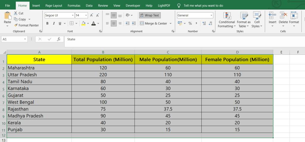
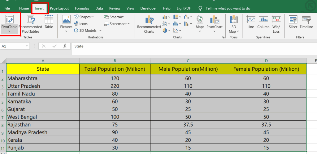
- 2nd:- Go to the “Insert” tab in Excel’s toolbar and click on the “PivotTable” button.
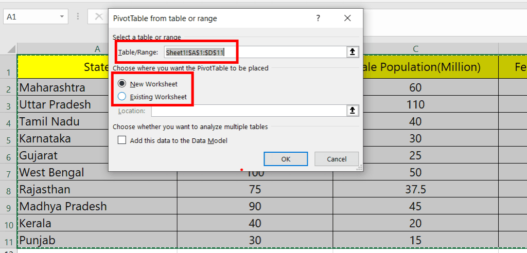
- 3rd:- In the dialog box that appears, choose where you want the Pivot Table to be placed (in a new worksheet or an existing one).
- 4th:- Drag and drop the desired fields from your dataset into the appropriate areas of the Pivot Table interface: “Rows,” “Columns,” “Values,” and “Filters.”
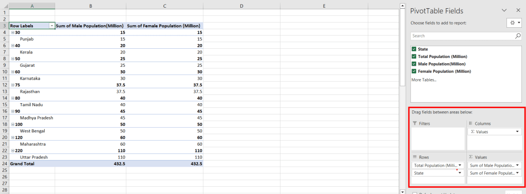
- 5th:- Customize your Pivot Table by rearranging fields, applying filters, adding calculations, and formatting as needed.
Free Download
Example of Pivot Table in Excel
Pivot Table in Excel is a game-changer when it comes to data analysis and reporting. They provide a dynamic and flexible way to transform raw data into insightful summaries, enabling users to uncover hidden patterns, trends, and relationships.
In this section, we will explore some real-life examples that showcase the versatility and effectiveness of Pivot Tables in various domains. From sales analysis to financial reporting, these examples will demonstrate how Pivot Table in Excel can simplify complex data sets and empower users to make informed decisions with ease. So, let’s dive into the world of Pivot Table examples and discover the endless possibilities they offer!
- Example 1: Sales Analysis
Let’s say you have a sales dataset with columns such as “Product,” “Region,” “Salesperson,” and “Quantity Sold.” By creating a Pivot Table, you can quickly analyze the sales data in various ways:
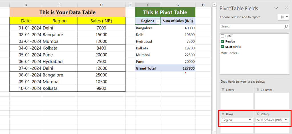
- Summarize total sales by region: Drag the “Region” field to the “Rows” area and the “Sales” field to the “Values” area. Excel will automatically calculate the total sales for each region.
- Compare sales by product and region: Place the “Product” field in the “Rows” area, the “Region” field in the “Columns” area, and the “Sales” field in the “Values” area. Excel will generate a matrix showing sales figures for each product by region.
- Analyze salesperson performance: Add the “Salesperson” field to the “Rows” area and the “Sales” field to the “Values” area. You can then sort or filter the data to identify top performers or underperformers.
Learn Excel
- Example 2: Financial Analysis
Pivot Table in Excel are not limited to sales analysis; they can be used in various domains, including finance. For instance, you can use Pivot Table in Excel to analyze financial data such as expenses, revenue, and profitability:
- Calculate total expenses by category: Drag the “Expense Category” field to the “Rows” area and the “Amount” field to the “Values” area. Excel will summarize expenses for each category.

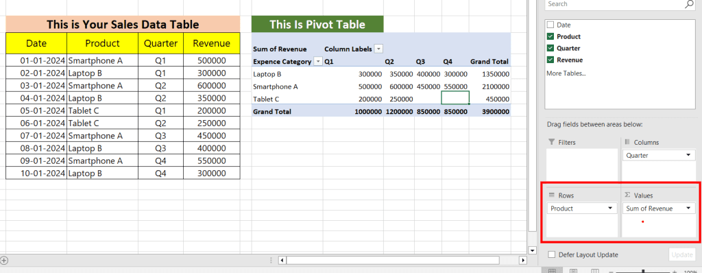
- Determine revenue by product and quarter: Place the “Product” field in the “Rows” area, the “Quarter” field in the “Columns” area, and the “Revenue” field in the “Values” area. Excel will provide a clear overview of revenue generated by each product during different quarters.
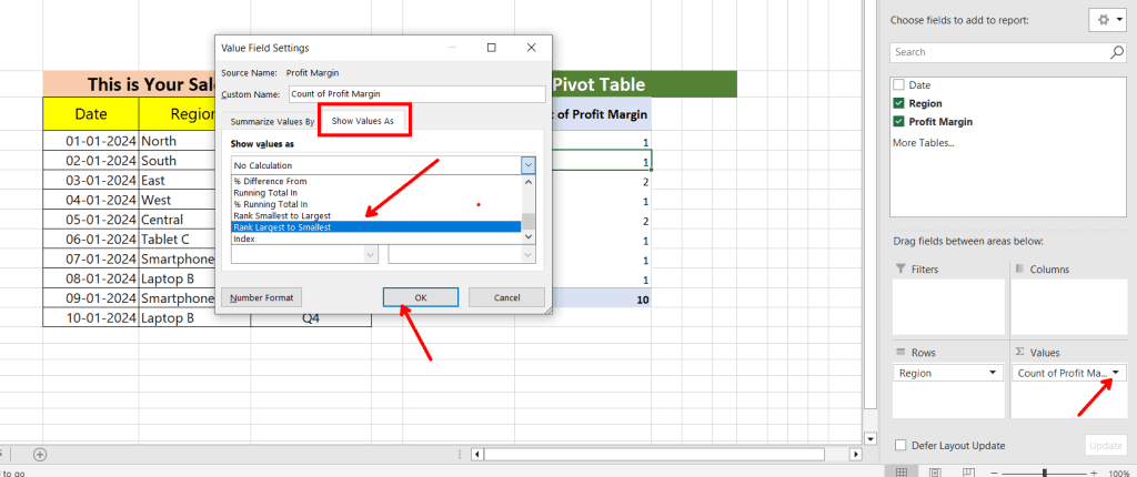
- Analyze profitability by region: Add the “Region” to Rows and “Profit Margin” fields to the Values. Then Click Arrow of the “Profit Margin” Field In Values Section, Click On “Value Field Settings” Option.
- You can then sort or filter data based on profit margins to identify regions with high or low profitability as shown in the below image.
Conclusion:
Pivot Table in Excel is an invaluable tool for data analysis, offering a simple yet powerful way to transform raw data into meaningful insights. By summarizing and manipulating large datasets, Pivot Tables enable users to uncover trends, patterns, and relationships that may otherwise go unnoticed. Whether you’re analyzing sales data, performing financial analysis, or exploring any other domain, Pivot Tables provide a dynamic and flexible solution.
With just a few clicks, you can create interactive reports, customize your analysis, and make informed decisions based on accurate and organized information. Pivot Tables allow you to slice and dice data, filter results, explore details behind the summaries, and visualize your findings through Pivot Charts. The ability to update automatically with new data ensures that your analysis remains up-to-date without any manual intervention.
Free Download
By mastering Pivot Table in Excel, you can streamline your data analysis process and save valuable time. You’ll be able to handle large datasets effortlessly, gain valuable insights with ease, and present your findings in a clear and concise manner. Whether you’re a business professional, analyst, or student, understanding how to leverage the power of Pivot Tables will undoubtedly enhance your analytical capabilities and contribute to better decision-making.
FAQs about Pivot Tables in Excel:
Q1: What is the advantage of using a Pivot Table?
A1: Pivot Tables offer several advantages, including the ability to summarize and analyze large datasets quickly, identify trends and patterns, create interactive reports, and easily update data as it changes.
Q2: Can I create a Pivot Table with multiple data sources?
A2: Yes, you can create a Pivot Table with multiple data sources. Excel allows you to consolidate data from different worksheets or workbooks into a single Pivot Table, providing a comprehensive view of your data.
Q3: Can I change the layout and appearance of a Pivot Table?
A3: Absolutely! Excel provides various customization options for Pivot Tables. You can rearrange fields, apply different formatting styles, add calculations, sort and filter data, and even create charts based on your Pivot Table results.
Cheat Sheets
Q4: Can I update my Pivot Table automatically when new data is added?
A4: Yes, you can set up your Pivot Table to update automatically when new data is added to the source range. Simply enable the “Refresh Data When Opening the File” option or use the “Refresh All” button to update your Pivot Table with the latest data.
Q5: Can I use functions like SUM or AVERAGE within a Pivot Table?
A5: Absolutely! Excel allows you to use various functions within a Pivot Table. You can perform calculations such as summing values, finding averages, calculating percentages, and more by adding calculated fields or using built-in functions within the Value area of your Pivot Table.
Q6: Can I filter my Pivot Table based on specific criteria?
A6: Yes, you can filter your Pivot Table based on specific criteria. Excel provides filtering options that allow you to include or exclude certain values, apply date filters, create custom filters, and even use slicers for interactive filtering.
Q7: Can I drill down into the details behind the summarized data in a Pivot Table?
A7: Absolutely! Excel allows you to drill down into the details behind your summarized data. By double-clicking on a cell within your Pivot Table, you can access the underlying data and explore the individual records that contribute to the summary.
How to use conditional formatting in excel for Dynamic Spreadsheets!
Excel Tips
Q8: Can I create Pivot Charts based on my Pivot Table?
A8: Yes, Excel offers the option to create Pivot Charts based on your Pivot Table. This allows you to visualize your data and gain further insights through various chart types, including column charts, line charts, bar charts, and more.
Q9: Can I share my Pivot Table with others who don’t have Excel?
A9: Yes, you can share your Pivot Table with others who don’t have Excel by saving it as a PDF or an image file. This way, they can view and analyze the summarized data without needing Excel installed on their devices.
Q10: Are there any limitations to using Pivot Tables in Excel?
A10: While Pivot Tables are highly versatile and powerful, they do have some limitations. For example, they may not handle extremely large datasets efficiently, and certain complex calculations may require additional formulas or functions outside of the Pivot Table. However, these limitations can often be overcome with creative solutions or alternative approaches in Excel.
Excel Trics

